Note:

This post assumes that you have a basic knowledge of recurrent neural networks (RNN) and are seeking for a more in-depth understanding of the mathematical description of the RNN and its most popular LSTM variants.

Recurrent neural networks (RNN) are a common approach to modelling sequential data as unlike its base form (the dense neural network), it can use its internal state to process input sequences of variable lengths. This makes them applicable to and more suitable for tasks such as speech recognition, machine translation, text-to-speech tasks, weather forecasting, etc.

This post describes:

• the basic structure of an RNN, and
• its most popular variant, the Long Short-term Memory (LSTM) cell.

Recurrent Neural Networks (RNN)

Mathematically, inputs to a neural network are vectors. The length of each input vector (or the number of dimensions of each vector) depends on the number of features you have. For a task like automatic speech recognition, your input features might be the Mel filter bank coefficients. The length of each input vector is thus the number of coefficients you use.

Consider an input sequence of length $T$, $\mathbf{x}_{1:T} = (\mathbf{x}_1, \ldots, \mathbf{x}_T)$, where $\mathbf{x}_t$ is a $d$-dimensional feature vector. Denote the output sequence of labels of length $U$ as $y_{1:U} = (y_1, \ldots, y_U)$ where $y_u$ takes the value of a symbol from a vocabulary $\mathcal{A}$ of size $K$, i.e. $y_u \in \mathcal{A}$. Note that $T$ is not necessarily equal to $U$ in general.

RNN is useful to model the mapping of $\mathbf{x}_{1:T}$ to $y_{1:U}$ when $T=U$, i.e. when the input and output sequences are of the same length. In the RNN, a hidden state vector $\mathbf{h}_t$ is introduced to encode and represent the previous inputs, $\mathbf{x}_{1:t}$, where $1 \leq t \leq T$. The figure below shows an RNN model unrolled in time, with the hidden state vector $\mathbf{h}_t$ depicted.

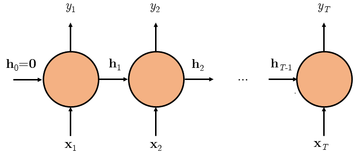
From the figure, at a time step $t$, $\mathbf{h}_{t-1}$ and $\mathbf{x}_t$ is used to calculate $\mathbf{h}_t$, as described by the recurrence relation in Equation \ref{eq: RNN 1}.

where $\mathbf{W}_{xh}$, $\mathbf{W}_{hh}$, $\mathbf{b}_{xh}$ and $\mathbf{b}_{hh}$ are trainable weight matrices and bias vectors, and $\phi(\cdot)$ is the activation function, typically the $tanh$ function. Notice from Equation \ref{eq: RNN 1} that $\mathbf{h}_t$ is in fact a function of all the input vectors up to time $t$, $\mathbf{x}_{1:t}$.

Apart from being passed on to the next time step, $t+1$, $\mathbf{h}_t$ is also used to predict the output value at time $t$. More precisely, $\mathbf{h}_t$ is used to compute the posterior probability of all the possible output values at time $t$ (i.e. $\text{P}(y_t = a|\mathbf{x}_{1:t}) \, \forall \, a \in \mathcal{A}$) as described in Equations \ref{eq: RNN 2} and \ref{eq: RNN 3}. The final output value $y_t$ is then predicted by sampling from the posterior probability $\text{P}(y_t|\mathbf{x}_{1:t})$.

Deep RNN model

RNNs can be stacked on top of each other, where the hidden vectors of an RNN become the input vectors of another RNN, forming a deep RNN model. Writing Equation \ref{eq: RNN 1} as $\mathbf{h}_t = \mathcal{F}_{\text{RNN}}(\mathbf{x}_{t}, \mathbf{h}_{t-1})$, a 2-hidden-layer RNN model can be written as:

where the superscript $(l)$ represents the $l$-th hidden layer.

An RNN is trained using gradient descent with error back-propagation through time (BPTT). The objective function is the cross entropy (CE) loss:

where $\mathbb{I}$ is the indicator function.

Note that the inner sum represents the usual cross entropy loss function in a multi-class classification problem. In RNN, this cross entropy loss is summed up across all time steps to get the final cross entropy loss for the entire input sequence.

Long Short-term Memory (LSTM)

As the input sequence grows longer (i.e. huge $T$), vanishing gradient becomes a problem in RNN and earlier input frames become less significant in the learning of the weights.

To address this problem, a variant known as the Long Short-term Memory cell (LSTM) was proposed in this paper. Three gate mechanisms are introduced to the RNN, as well as a separate cell state $\mathbf{c}_t$ on top of the existing hidden state $\mathbf{h}_t$. Equations \ref{eq: LSTM 1} to \ref{eq: LSTM 3} describe the computation of the input, forget and output gates using the input vector $\mathbf{x}_t$ and the hidden state vector $\mathbf{h}_{t-1}$

where $\mathbf{W}$'s and $\mathbf{b}$'s are trainable weights and biases.

The newly introduced cell state $\mathbf{c}_t$ is calculated using the cell state from the previous time step $\mathbf{c}_{t-1}$, the hidden state from the previous step ${\mathbf{h}_{t-1}}$ and the input vector at the current step ${\mathbf{x}_t}$. Equation \ref{eq: LSTM 4} computes the cell state while equation \ref{eq: LSTM 5} computes the hidden state from the cell state.

where the $\mathbf{W}$'s and $\mathbf{b}$'s are also trainable weights and biases, and $\odot$ indicates the element-wise product operation.

Like with the RNN, $\mathbf{h}_t$ is used to calculate the output probability of each token value at time step $t$:

Like the RNN, the LSTM can be trained by optimising the CE loss using gradient descent with error BPTT. They can also be stacked to form deeper architectures. Writing equations \ref{eq: LSTM 1} to \ref{eq: LSTM 5} as $\mathbf{h}_t = \mathcal{F}_{\text{LSTM}}(\mathbf{x}_{t}, \mathbf{h}_{t-1}, \mathbf{c}_{t-1})$, a 2-hidden-layer LSTM can be described with:

To learn more about the LSTM and to gain an intuition about the cell state and the various gates, I highly suggest reading this classic post from Colah’s blog.

Bidirectional LSTM (BLSTM)

With RNNs and LSTMs, there is an inherent assumption that at time $t$, only the input vectors up to time $t$ is available. In other words, only $\mathbf{x}_{1:t}$ is available and not $\mathbf{x}_{t+1:T}$ because they are in the future. Therefore, the output at time $t$, $y_t$, can only be predicted using past information. An example is streaming speech recognition where transcriptions are generated in real-time. The system cannot predict the text output for something that it has not heard.

In some applications, however, the entire input sequence $\mathbf{x}_{1:T}$ might be available at prediction time $t$. An example is when transcriptions are not required to be generated in real-time but only after the fact. In this case the entire speech is available for speech recognition, and the prediction of $y_t$ can be based on both the past and future information.

For these applications, a bidirectional LSTM (BLSTM) model can be used to exploit future context while modelling the posterior probability of $y_t$. In BLSTM, two LSTMs are used, each unrolling in opposite directions in time starting from the first and the last inputs, $\mathbf{x}_1$ and $\mathbf{x}_T$, respectively. Two sets of hidden and cell state vectors are computed recurrently: one set in the forward direction $(\mathbf{h}_{1:T}^f, \mathbf{c}_{1:T}^f)$ starting from the first input, one set in the backward direction $(\mathbf{h}_{1:T}^b, \mathbf{c}_{1:T}^b)$ starting from the last input. At each time $t$, both hidden vectors, $\mathbf{h}_{t}^f$ and $\mathbf{h}_{t}^b$, are combined to compute the final hidden vector, $\mathbf{h}_{t}$. Equations \ref{eq: BLSTM 1} to \ref{eq: BLSTM 4} describe this.

where $[\mathbf{a}; \mathbf{b}]$ represents a concatenation of vectors $\mathbf{a}$ and $\mathbf{b}$.

To understand the equations better, equation \ref{eq: BLSTM 1} is the usual LSTM operation on an input sequence $\mathbf{x}_{1:T}$. Now, duplicate the input sequence and flip it around so that it goes in the opposite direction of the original sequence, $\mathbf{x}_{T:1}$. Equation \ref{eq: BLSTM 2} is basically another LSTM operation applied to this flipped input sequence. The hidden vector from equation \ref{eq: BLSTM 1}, $\mathbf{h}_t^f$, represents the past context while the hidden vector from equation \ref{eq: BLSTM 2}, $\mathbf{h}_t^b$, represents the future context. Both the past and future contexts are combined in equation \ref{eq: BLSTM 3} to give a more comprehensive hidden vector $\mathbf{h}_t$ to allow for a more accurate prediction of the output posterior probability than a typical unidirectional LSTM or RNN.

Future context, although helpful, comes at the cost of latency. With a bidirectional structure, a token $y_t$ can only be predicted after the entire input sequence is read. This makes it less useful for applications which require low latency like streaming or real-time prediction tasks.

Uni-LSTM with context

To reduce latency and yet exploit future context of the input sequence, the unidirectional LSTM ($\mathbf{h}_t = \mathcal{F}_{\text{LSTM}}(\mathbf{x}_{1:t})$) can be modified so that a token $y_t$ is predicted after a time offset $\delta$, i.e. at the ($t+\delta$)-th time step. This allows the model to have $\delta$ future input context to make a prediction. In other words, the model is able to look $\delta$ steps ahead before making a prediction. By controlling $\delta$, the trade-off between amount of future context and latency can be controlled. Essentially, $\delta = 0$ gives you the original unidirectional LSTM and $\delta = T - t$ effectively gives you a bidirectional LSTM.

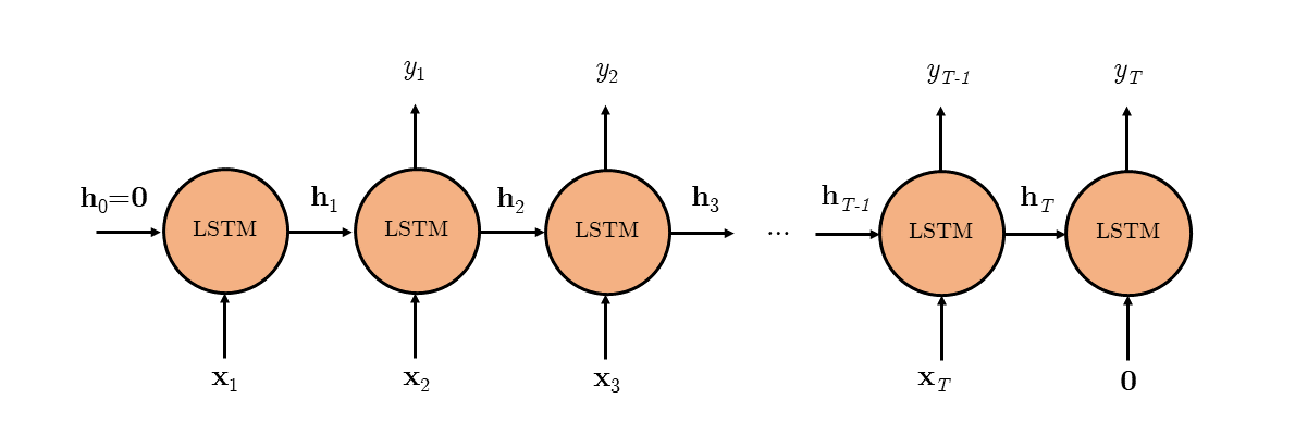
To achieve this, $\delta$ all-zero vectors are appended to the input sequence $\mathbf{x}_{1:T}$. No prediction is made at the first $\delta$ time steps, with the first prediction made on the $(\delta + 1)$-th time step. Equations \ref{eq: LSTM 1} to \ref{eq: LSTM 6} then become

The figure below shows a unidirectional LSTM with $\delta=1$ future context frame unrolled in time. Note the all-zero vector after the last original input $\mathbf{x}_T$. An output token $y_t$ is only predicted at the ($t+1$)-th time step, allowing the model to look one step ahead before making the prediction.

Note that although setting $\delta = T - t$ means predicting the output with the entire input sequence available, thus making it conceptually identical to the BLSTM, notice that the architecture is different! In this uni-LSTM with context architecture, there is only one LSTM model moving in the forward direction, whereas in BLSTM there are two, one in each direction.

LSTM Projected Architecture (LSTMP)

Although LSTMs have the added advantage of reducing vanishing gradient, they have a huge number of trainable parameters due to the computation of the gates. (Remember all the $\mathbf{W}$'s and $\mathbf{b}$'s?) To reduce the computation complexity of learning LSTM models, an LSTM projected architecture (LSTMP) was proposed in this paper.

In this architecture, a linear projected layer is added after the recurrent LSTM layer to project the hidden vector $\mathbf{h}_t$ down to a lower number of dimensions. This reduces the number of trainable weights and hence the complexity while minimising the trade-off with modelling power. Equations \ref{eq: LSTMP 1} to \ref{eq: LSTMP 3} describe the LSTMP architecture.

where $\mathbf{\tilde{h}}_t$ is the original hidden vector, and $\mathbf{h}_t$ is now the projected hidden vector. Note that in equation \ref{eq: LSTMP 1}, the projected hidden vector is used to compute the hidden vector instead of the original hidden vector.

Conclusion

1. Recurrent neural networks (RNNs) are commonly used in sequence modelling due to a hidden state being introduced to encapsulate past information in a sequence.
2. Long Short-term Memory cells (LSTMs) introduce 3 gate mechanisms and an additional cell state to address the issue of vanishing gradient with RNN.
3. Some variants of LSTMs include the bidirectional LSTM, uni-LSTM with context, and the LSTMP architectures.

Author: Chia Jing Heng (andreusjh99)